A more quantitative approach to rugby union
Territorial Game?
Collision sports are territorial games. Conventional wisdom suggests a strong, positive correlation between territory gained and tries/points scored. Empirical evidence, as depicted
in the graph below, begs to differ. The relationship between yardage gained and points scored in Rugby Union is vaguer than it is in American football, a sport that apparently
gave birth to this metric.
I’ve been collecting
the data on how the ball has travelled across the vertical zones. It’s just an approximation; it’s not perfect, but since the GPS/tracker data are not available,
the proxy is accurate enough. (For some post-match reports, I use pixels to calculate the exact position, but the data collection is extremely time consuming). In the figure below, tries
(left panel) and points scored are plotted against the percentage of total possessions when the ball travelled forwards. The points are randomly scattered over a wide area; no trend fits the
data reasonably well. It’s still possible, however, to interpret the relationship. That’s where statistics comes in handy.
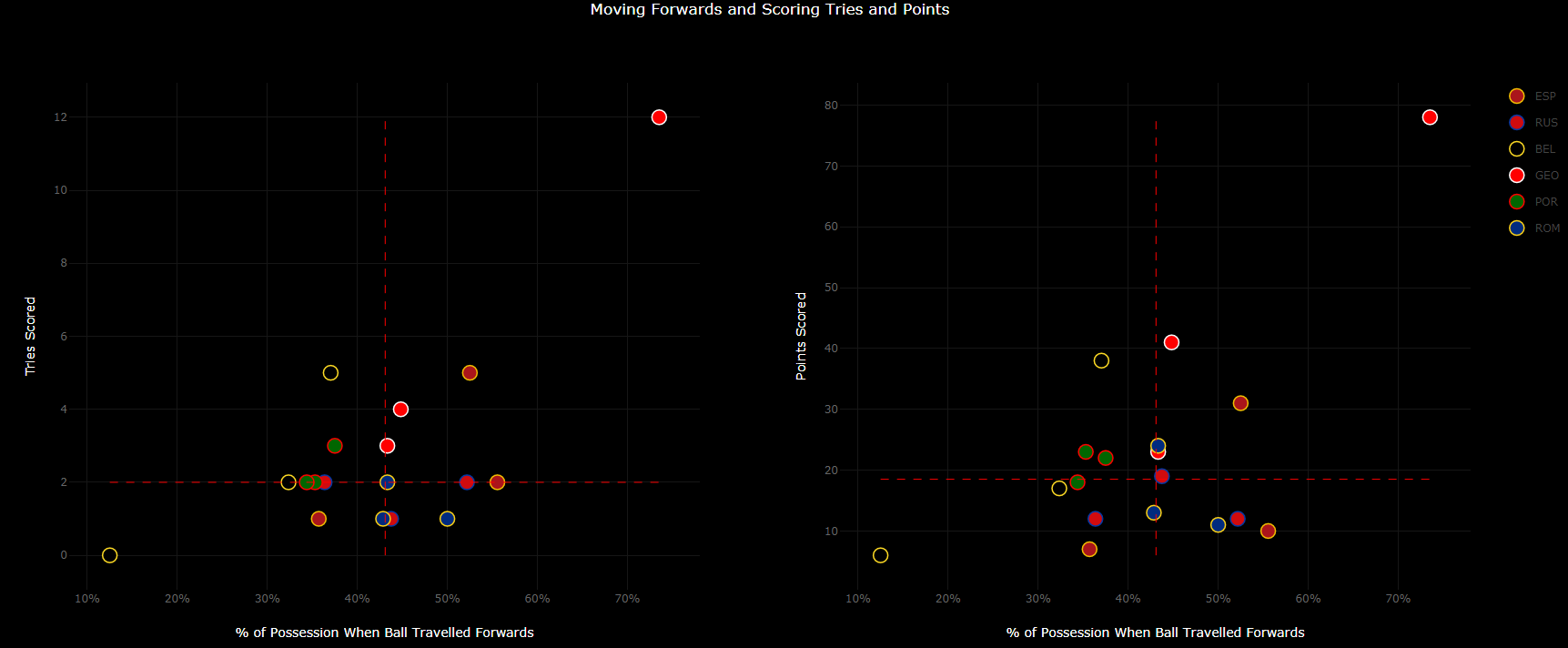
The graph’s surface is split into four quadrants by red dashed lines marking the respective medians. Why medians? When a team scores 12 tries and moves forwards in nearly 75% of its possessions,
the numbers clearly break the observed pattern. Arithmetic average, especially when the sample size is small, would be affected by the irregularity. The median marks the half-way of the sample
points and hence is more resilient to outlier than the arithmetic average. The quadrants have a rather intuitive interpretation. Dominant offences are to be found in the first quadrant. They
regularly march up the field and score more points than other teams. There are five markers in this region, not surprisingly three of them are red-white-coloured. Teams frequently gaining territory
but experiencing problems with turning opportunities into points are in the fourth quadrant. Falling into this quadrant doesn’t necessarily mean to lose a match, but all teams in this quadrant have
indeed lost their games, and so have the teams in the third quadrant. The most effective offences are in the second quadrant, as they gained less territory but put more point on the scoreboard. There
are only three markers in this quadrant. Two of them indicate a team freshly promoted to Europe’s second six.
Now let’s take a closer look at Los Leones and their Iberian neighbour. Portugal’s attack has been surprisingly consistent in terms of both scoring and moving across the vertical zones. The latter,
despite two wins, is fairly below the tournament median. Only Belgium have experienced more problems with gaining territory. Yet, Os Lobos have managed to score above the REC2020 median twice.

What’s the secret of Portugal’s attacking effectiveness? My guess would be speed and the width game. Their first try scored against Romania offers a good example. The attacking line-out in Opp 10-22 led to a
sequence of four passes, a retained grubber, and a try. The time of controlled possession for this platform was only 13 seconds.

In a sharp contrast to the Wolves, Los Leones hit three different quadrants in three different matches. The well-deserved win in the season opener in Sochi is marked by the entry in the much desired
first quadrant. The third round defeat against the Oaks is to be found in the third quadrant. Spain consequently gained territory against Russia, moving forwards in 53% of their possessions. In Botosani,
the ratio dropped to 36%.
The Defence
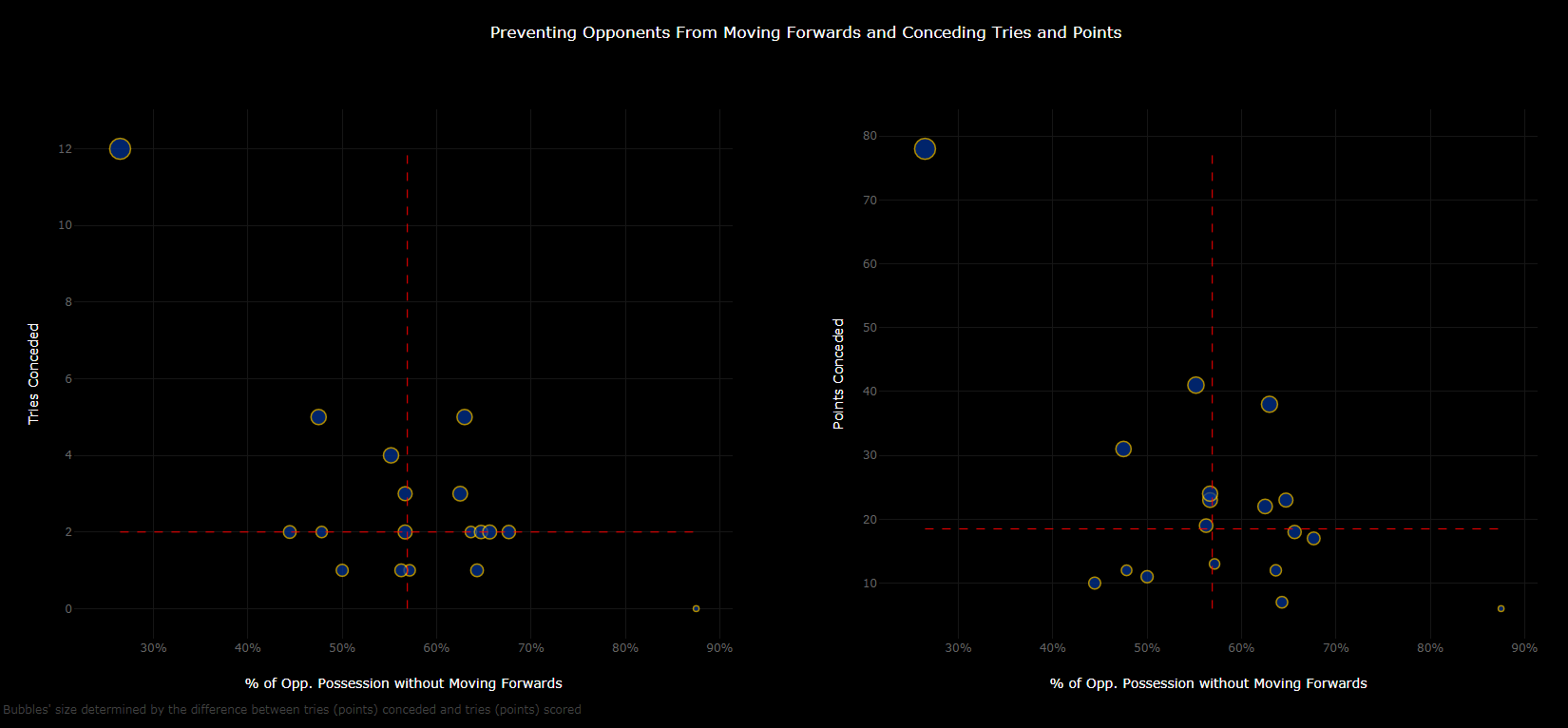
I created a similar graph for the defence. The bubbles mark the percentage of opponent possessions without moving forwards [X-axis] and tries and points conceded [Y-axis].
Bubble size varies and is determined by the difference between tries (points) scored and conceded. The one in the bottom-right corner, hardly visible, represents Georgia in round 3. Again,
I marked the medians, but this time I decided to apply slightly more sophisticated procedures to trace out the relationship between territory (or rather not losing it) and conceding tries.
I ran a simple model with only three explanatory variables: home/away, defensive penalties, and percentage of stopped offensive possessions (henceforth: stops). The applied method
was the Bayesian additive regression trees (BART, scroll down for some technicalities). I’d be more than happy to regress the number of tries conceded against a much larger set of explanatory
variables, but there aren’t any official statistics for REC matches, and I haven’t collected other defensive metrics like the tackle completion rate or defenders beaten.
Bear in mind that 3 rounds of REC have created merely 18 observations. It’s not much. In fact, the sample is extremely small. Despite this limitation, the model fits the data rather well (66%).
Which variable turned out to be the most important? Assuming that the total importance is 100%, the home/away, defensive penalties, and stops accounts for 22%, 37%, and 41%, respectively. The stops
are most important, but the penalties don’t lag behind too much. How do the variables affect the number of tries conceded? For stops and penalties, I assumed 5 hypothetical scenarios: what if a team achieved
max, 75% of max, median, 25% of max, and min of stop percentage (of conceded penalties). Not surprisingly, for home/away there’s only two.
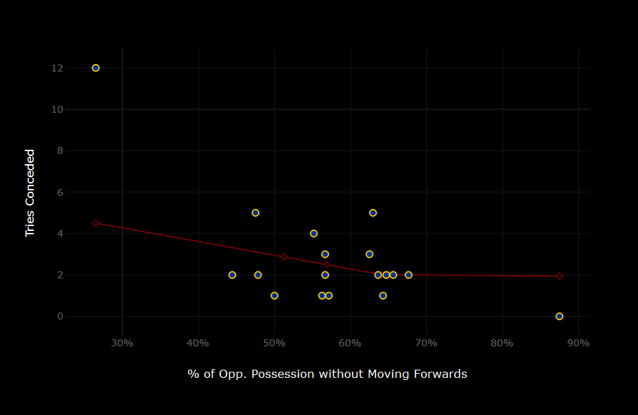
The burgundy line depicts the results for stops. The slope is steep between the min stops and 25th quantile (in other words: 25% of all stops is found below 51.3%), but then it becomes flat. If a team produces the stop
percentage below 45%, it’s very like that the team will concede 4 tries. Despite a huge difference between median stops (56.9%) and max stops (87.5%), the expected number of tries conceded for these percentages is 2.5
and 1.9. The varying slope captures an important feature of the territorial game – a defensive effort won’t be rewarded proportionally across the entire range of stops.
More importantly, the expected number of conceded tries falls below 2 when teams’ stopping percentage is 64.5%. That’s lots and lots of stops, but Romania (R3), Belgium (R1), Russia (R3), Portugal (R1) and obviously
Georgia (R3) managed to achieve it. This metric offers an additional insight into explaining the surprising upsets in round 3 – Romania defeating Spain and Russia winning against Portugal. (At least I found them
surprising). The Oaks and the Bears allowed their opponents to move forwards in 36% and 34% of possessions, respectively.
I also ran the simulations for the number of defensive penalties and home/away dummy (home = 1, away = 0). It turned out that the defensive penalties didn’t have much impact on the tries conceded, nor was the relationship
monotonic. The REC hosts are expected to concede one try less (2.1) than the guests (3.1).
Summing up, forcing an opponent backwards or at least stopping them in the same vertical zone the possession started seems to be an important factor in predicting how many tries the defence is going to concede. It’s much
more important when the stopping percentage is below the tournament median, however, than when it is above it. As maintaining a good line speed for 80 minutes is a rare commodity in the European T2 rugby, a bend-don’t-break
defence might offer a good alternative. Especially, when the width game doesn’t function perfectly.
Technical Details
The figures have been prepared in plotly. A script is
available here. The colours in lines 32-35 are official colours of the national
flags. To regress the BART model, I employed
bartMachine R package.
I experimented with the number of trees (between 10 and 50) and also varied other hyperparameters in order to minimise the forecast errors. Please note
that I assumed the beta parameter to be equal to 1 (the literature suggests 2). I set the number of burn-in and post-burn-in to 500 and 5000, respectively. The diagnostics panel shows:
[1] L1 – sum of absolute errors = 17.79. It means that the total (absolute value of the) difference between actual and predicted tries conceded was nearly 18. A lion’s share is
accounted for the outstanding offensive power of the Lelos . The model failed to expect 12 tries conceded by the Black Devils (prediction = 6), but didn’t you?
[2] L2 – sum of squared errors = 42.75.
[3] rmse – root mean square error = 1.54. RMSE measures the average spread of prediction errors.
[4] pseudo R^2 = 0.647. Decent fit, but as I mentioned it before, there’s a danger of overfitting. After setting the beta-coefficient to 2, the pseudo R^2 dropped to 0.475,
but the k-fold cross-validation didn’t indicate any considerable improvement.
[5] properties of the residual – the desired distribution in normal with zero-valued mean. The latter property is satisfied, the former, due to large heteroskedasticity
generated by the Georgia-vs-Belgium match, is not.
Again, please notice that this is just a preliminary analysis. I will update the results after the next rounds of REC 2020.